KD-Trees

A k-d tree (k-dimensional tree) is a binary search tree used to organize points in k-dimensional space. It supports efficient range and nearest-neighbor searches by recursively dividing space along alternating axes.

The first split (e.g., x-axis) creates two regions.
Each region is then split along the next axis (e.g., y-axis).
Final split occurs along the z-axis (or next axis in higher dimensions).
This creates compact, axis-aligned subregions ideal for search.

Construction

At each level, select axis = depth % k. Sort all points by that axis, then pick the median to split the space for balance. Recursively build left and right subtrees.


// Recursive function to build a k-d tree from an array of points
function kdtree(points, depth) {
  const k = points[0].length;
  const axis = depth % k;

  points.sort((a, b) => a[axis] - b[axis]);

  const medianIdx = Math.floor(points.length / 2);
  const node = {};
  node.point = points[medianIdx];
  node.left = (medianIdx > 0) ? kdtree(points.slice(0, medianIdx), depth + 1) : null;
  node.right = (medianIdx + 1 < points.length) ? kdtree(points.slice(medianIdx + 1), depth + 1) : null;
  return node;
}

Complexity

Operation	Average	Worst
Search	O(log n)	O(n)
Insert	O(log n)	O(n)
Delete	O(log n)	O(n)
Space	O(n)	O(n)

Insertion & Deletion

Insertion compares the new point along the current axis at each level and places it as a leaf. Deletion may involve replacing the node with the subtree’s minimum on that axis, then rebalancing the subtree.

Balancing

KD-Trees avoid tree rotations. Balance is handled during construction using median splits. For dynamic data, K-D-B trees or periodic rebuilding maintain balance.

Nearest-Neighbor Search

Recursively follow the split axis down to a leaf node.
Track and update the nearest neighbor based on squared distance.
If the hypersphere intersects the split plane, explore both subtrees.
Use squared Euclidean distance to avoid square root calculations.

KD-Tree Nearest Neighbor Search Demo

Enter query point coordinates and click "Find Nearest Point" to see the nearest neighbor in the KD-Tree.

Query X: Query Y:

Locality Sensitive Hashing (LSH)

Locality Sensitive Hashing (LSH) is a dimensionality reduction technique used to efficiently find approximate nearest neighbors in high-dimensional spaces. Unlike traditional hashing, LSH is designed so that similar inputs are mapped to the same buckets with a higher probability than dissimilar ones. This allows for scalable and efficient similarity search without exhaustive comparisons.

LSH works by constructing multiple hash functions based on a chosen distance metric, such as cosine similarity or Jaccard similarity. These hash functions are applied to each input vector, and the results are used to index the vector into multiple hash tables. During a query, the input vector is hashed in the same way, and only the entries in the matching buckets are considered for comparison.

For example, in a system with one million image vectors, each of 128 dimensions, instead of comparing a new image with all one million vectors, LSH hashes the image vector and searches only in the relevant buckets. This drastically reduces the number of comparisons needed.

LSH is widely applied in tasks such as near-duplicate detection of images and videos, document similarity matching, plagiarism detection, and recommendation systems.

The diagram below illustrates the core idea: similar vectors are more likely to fall into the same buckets across multiple hash tables.

LSH diagram illustrating how similar vectors land in the same bucket

Trie Data Structures

A Trie (prefix tree) is a tree-based data structure used to efficiently store and retrieve strings. It is especially useful for prefix-based queries.

Each node represents a character. The path from the root to a node represents a prefix. This structure allows efficient lookups, insertions, and deletions.

Applications: Autocomplete, Spell Checking, IP Routing, etc.

Pseudocode

Pathfinding Algorithms: DFS, BFS, Dijkstra, A*

This section compares core pathfinding algorithms with side-by-side animation. Click any button to see how each algorithm explores nodes.

1. DFS (Depth-First Search)

DFS explores one branch deeply before backtracking. In this case, it follows A → B → D → G. It chooses this path because it dives into B, then continues to D, and finally to G, even though it is not the optimal path cost-wise.

DFS(G, u)
  u.visited = true
  for each v ∈ G.Adj[u]
    if v.visited == false
      DFS(G, v)

init()
  for each u ∈ G
    u.visited = false
  for each u ∈ G
    DFS(G, u)

2. BFS (Breadth-First Search)

BFS explores level-by-level. It finds A → B → E → G as the shortest path by number of edges, not cost. It explores neighbors before going deeper, making it optimal for unweighted graphs.

Create a queue Q
Mark v as visited and put v into Q

while Q is not empty:
  remove the head u of Q
  for each unvisited neighbour w of u:
    mark w as visited
    enqueue w into Q

3. Dijkstra’s Algorithm

Dijkstra selects the lowest cumulative cost at every step. It also finds A → B → E → G as the minimum-cost path (cost = 7). It avoids A → C → F → G and A → B → D → G as they are more expensive.

function dijkstra(G, S)
    for each vertex V in G
        distance[V] <- infinite
        previous[V] <- NULL
        If V != S, add V to Priority Queue Q
    distance[S] <- 0
	
    while Q IS NOT EMPTY
        U <- Extract MIN from Q
        for each unvisited neighbour V of U
            tempDistance <- distance[U] + edge_weight(U, V)
            if tempDistance < distance[V]
                distance[V] <- tempDistance
                previous[V] <- U
    return distance[], previous[]

4. A* Algorithm

A* uses both actual cost and estimated cost (heuristic). With heuristics: A(6), B(4), E(2), it selects A → B → E → G as the optimal route combining cost-so-far and estimated cost to goal (f(n) = g(n) + h(n)). The heuristics are shown on the graph nodes.

// A C++ Program to implement A* Search Algorithm
#include 
using namespace std;

#define ROW 9
#define COL 10

// Creating a shortcut for int, int pair type
typedef pair Pair;

// Creating a shortcut for pair> type
typedef pair > pPair;

// A structure to hold the necessary parameters
struct cell {
    // Row and Column index of its parent
    // Note that 0 <= i <= ROW-1 & 0 <= j <= COL-1
    int parent_i, parent_j;
    // f = g + h
    double f, g, h;
};

// A Utility Function to check whether given cell (row, col)
// is a valid cell or not.
bool isValid(int row, int col)
{
    // Returns true if row number and column number
    // is in range
    return (row >= 0) && (row < ROW) && (col >= 0)
           && (col < COL);
}

// A Utility Function to check whether the given cell is
// blocked or not
bool isUnBlocked(int grid[][COL], int row, int col)
{
    // Returns true if the cell is not blocked else false
    if (grid[row][col] == 1)
        return (true);
    else
        return (false);
}

// A Utility Function to check whether destination cell has
// been reached or not
bool isDestination(int row, int col, Pair dest)
{
    if (row == dest.first && col == dest.second)
        return (true);
    else
        return (false);
}

// A Utility Function to calculate the 'h' heuristics.
double calculateHValue(int row, int col, Pair dest)
{
    // Return using the distance formula
    return ((double)sqrt(
        (row - dest.first) * (row - dest.first)
        + (col - dest.second) * (col - dest.second)));
}

// A Utility Function to trace the path from the source
// to destination
void tracePath(cell cellDetails[][COL], Pair dest)
{
    printf("\nThe Path is ");
    int row = dest.first;
    int col = dest.second;

    stack Path;

    while (!(cellDetails[row][col].parent_i == row
             && cellDetails[row][col].parent_j == col)) {
        Path.push(make_pair(row, col));
        int temp_row = cellDetails[row][col].parent_i;
        int temp_col = cellDetails[row][col].parent_j;
        row = temp_row;
        col = temp_col;
    }

    Path.push(make_pair(row, col));
    while (!Path.empty()) {
        pair p = Path.top();
        Path.pop();
        printf("-> (%d,%d) ", p.first, p.second);
    }

    return;
}

// A Function to find the shortest path between
// a given source cell to a destination cell according
// to A* Search Algorithm
void aStarSearch(int grid[][COL], Pair src, Pair dest)
{
    // If the source is out of range
    if (isValid(src.first, src.second) == false) {
        printf("Source is invalid\n");
        return;
    }

    // If the destination is out of range
    if (isValid(dest.first, dest.second) == false) {
        printf("Destination is invalid\n");
        return;
    }

    // Either the source or the destination is blocked
    if (isUnBlocked(grid, src.first, src.second) == false
        || isUnBlocked(grid, dest.first, dest.second)
               == false) {
        printf("Source or the destination is blocked\n");
        return;
    }

    // If the destination cell is the same as source cell
    if (isDestination(src.first, src.second, dest)
        == true) {
        printf("We are already at the destination\n");
        return;
    }

    // Create a closed list and initialise it to false which
    // means that no cell has been included yet This closed
    // list is implemented as a boolean 2D array
    bool closedList[ROW][COL];
    memset(closedList, false, sizeof(closedList));

    // Declare a 2D array of structure to hold the details
    // of that cell
    cell cellDetails[ROW][COL];

    int i, j;

    for (i = 0; i < ROW; i++) {
        for (j = 0; j < COL; j++) {
            cellDetails[i][j].f = FLT_MAX;
            cellDetails[i][j].g = FLT_MAX;
            cellDetails[i][j].h = FLT_MAX;
            cellDetails[i][j].parent_i = -1;
            cellDetails[i][j].parent_j = -1;
        }
    }

    // Initialising the parameters of the starting node
    i = src.first, j = src.second;
    cellDetails[i][j].f = 0.0;
    cellDetails[i][j].g = 0.0;
    cellDetails[i][j].h = 0.0;
    cellDetails[i][j].parent_i = i;
    cellDetails[i][j].parent_j = j;

    /*
     Create an open list having information as-
     >
     where f = g + h,
     and i, j are the row and column index of that cell
     Note that 0 <= i <= ROW-1 & 0 <= j <= COL-1
     This open list is implemented as a set of pair of
     pair.*/
    set openList;

    // Put the starting cell on the open list and set its
    // 'f' as 0
    openList.insert(make_pair(0.0, make_pair(i, j)));

    // We set this boolean value as false as initially
    // the destination is not reached.
    bool foundDest = false;

    while (!openList.empty()) {
        pPair p = *openList.begin();

        // Remove this vertex from the open list
        openList.erase(openList.begin());

        // Add this vertex to the closed list
        i = p.second.first;
        j = p.second.second;
        closedList[i][j] = true;

        /*
         Generating all the 8 successor of this cell

             N.W   N   N.E
               \   |   /
                \  |  /
             W----Cell----E
                  / | \
                /   |  \
             S.W    S   S.E

         Cell-->Popped Cell (i, j)
         N -->  North       (i-1, j)
         S -->  South       (i+1, j)
         E -->  East        (i, j+1)
         W -->  West           (i, j-1)
         N.E--> North-East  (i-1, j+1)
         N.W--> North-West  (i-1, j-1)
         S.E--> South-East  (i+1, j+1)
         S.W--> South-West  (i+1, j-1)*/

        // To store the 'g', 'h' and 'f' of the 8 successors
        double gNew, hNew, fNew;

        //----------- 1st Successor (North) ------------

        // Only process this cell if this is a valid one
        if (isValid(i - 1, j) == true) {
            // If the destination cell is the same as the
            // current successor
            if (isDestination(i - 1, j, dest) == true) {
                // Set the Parent of the destination cell
                cellDetails[i - 1][j].parent_i = i;
                cellDetails[i - 1][j].parent_j = j;
                printf("The destination cell is found\n");
                tracePath(cellDetails, dest);
                foundDest = true;
                return;
            }
            // If the successor is already on the closed
            // list or if it is blocked, then ignore it.
            // Else do the following
            else if (closedList[i - 1][j] == false
                     && isUnBlocked(grid, i - 1, j)
                            == true) {
                gNew = cellDetails[i][j].g + 1.0;
                hNew = calculateHValue(i - 1, j, dest);
                fNew = gNew + hNew;

                // If it isn’t on the open list, add it to
                // the open list. Make the current square
                // the parent of this square. Record the
                // f, g, and h costs of the square cell
                //                OR
                // If it is on the open list already, check
                // to see if this path to that square is
                // better, using 'f' cost as the measure.
                if (cellDetails[i - 1][j].f == FLT_MAX
                    || cellDetails[i - 1][j].f > fNew) {
                    openList.insert(make_pair(
                        fNew, make_pair(i - 1, j)));

                    // Update the details of this cell
                    cellDetails[i - 1][j].f = fNew;
                    cellDetails[i - 1][j].g = gNew;
                    cellDetails[i - 1][j].h = hNew;
                    cellDetails[i - 1][j].parent_i = i;
                    cellDetails[i - 1][j].parent_j = j;
                }
            }
        }

        //----------- 2nd Successor (South) ------------

        // Only process this cell if this is a valid one
        if (isValid(i + 1, j) == true) {
            // If the destination cell is the same as the
            // current successor
            if (isDestination(i + 1, j, dest) == true) {
                // Set the Parent of the destination cell
                cellDetails[i + 1][j].parent_i = i;
                cellDetails[i + 1][j].parent_j = j;
                printf("The destination cell is found\n");
                tracePath(cellDetails, dest);
                foundDest = true;
                return;
            }
            // If the successor is already on the closed
            // list or if it is blocked, then ignore it.
            // Else do the following
            else if (closedList[i + 1][j] == false
                     && isUnBlocked(grid, i + 1, j)
                            == true) {
                gNew = cellDetails[i][j].g + 1.0;
                hNew = calculateHValue(i + 1, j, dest);
                fNew = gNew + hNew;

                // If it isn’t on the open list, add it to
                // the open list. Make the current square
                // the parent of this square. Record the
                // f, g, and h costs of the square cell
                //                OR
                // If it is on the open list already, check
                // to see if this path to that square is
                // better, using 'f' cost as the measure.
                if (cellDetails[i + 1][j].f == FLT_MAX
                    || cellDetails[i + 1][j].f > fNew) {
                    openList.insert(make_pair(
                        fNew, make_pair(i + 1, j)));
                    // Update the details of this cell
                    cellDetails[i + 1][j].f = fNew;
                    cellDetails[i + 1][j].g = gNew;
                    cellDetails[i + 1][j].h = hNew;
                    cellDetails[i + 1][j].parent_i = i;
                    cellDetails[i + 1][j].parent_j = j;
                }
            }
        }

        //----------- 3rd Successor (East) ------------

        // Only process this cell if this is a valid one
        if (isValid(i, j + 1) == true) {
            // If the destination cell is the same as the
            // current successor
            if (isDestination(i, j + 1, dest) == true) {
                // Set the Parent of the destination cell
                cellDetails[i][j + 1].parent_i = i;
                cellDetails[i][j + 1].parent_j = j;
                printf("The destination cell is found\n");
                tracePath(cellDetails, dest);
                foundDest = true;
                return;
            }

            // If the successor is already on the closed
            // list or if it is blocked, then ignore it.
            // Else do the following
            else if (closedList[i][j + 1] == false
                     && isUnBlocked(grid, i, j + 1)
                            == true) {
                gNew = cellDetails[i][j].g + 1.0;
                hNew = calculateHValue(i, j + 1, dest);
                fNew = gNew + hNew;

                // If it isn’t on the open list, add it to
                // the open list. Make the current square
                // the parent of this square. Record the
                // f, g, and h costs of the square cell
                //                OR
                // If it is on the open list already, check
                // to see if this path to that square is
                // better, using 'f' cost as the measure.
                if (cellDetails[i][j + 1].f == FLT_MAX
                    || cellDetails[i][j + 1].f > fNew) {
                    openList.insert(make_pair(
                        fNew, make_pair(i, j + 1)));

                    // Update the details of this cell
                    cellDetails[i][j + 1].f = fNew;
                    cellDetails[i][j + 1].g = gNew;
                    cellDetails[i][j + 1].h = hNew;
                    cellDetails[i][j + 1].parent_i = i;
                    cellDetails[i][j + 1].parent_j = j;
                }
            }
        }

        //----------- 4th Successor (West) ------------

        // Only process this cell if this is a valid one
        if (isValid(i, j - 1) == true) {
            // If the destination cell is the same as the
            // current successor
            if (isDestination(i, j - 1, dest) == true) {
                // Set the Parent of the destination cell
                cellDetails[i][j - 1].parent_i = i;
                cellDetails[i][j - 1].parent_j = j;
                printf("The destination cell is found\n");
                tracePath(cellDetails, dest);
                foundDest = true;
                return;
            }

            // If the successor is already on the closed
            // list or if it is blocked, then ignore it.
            // Else do the following
            else if (closedList[i][j - 1] == false
                     && isUnBlocked(grid, i, j - 1)
                            == true) {
                gNew = cellDetails[i][j].g + 1.0;
                hNew = calculateHValue(i, j - 1, dest);
                fNew = gNew + hNew;

                // If it isn’t on the open list, add it to
                // the open list. Make the current square
                // the parent of this square. Record the
                // f, g, and h costs of the square cell
                //                OR
                // If it is on the open list already, check
                // to see if this path to that square is
                // better, using 'f' cost as the measure.
                if (cellDetails[i][j - 1].f == FLT_MAX
                    || cellDetails[i][j - 1].f > fNew) {
                    openList.insert(make_pair(
                        fNew, make_pair(i, j - 1)));

                    // Update the details of this cell
                    cellDetails[i][j - 1].f = fNew;
                    cellDetails[i][j - 1].g = gNew;
                    cellDetails[i][j - 1].h = hNew;
                    cellDetails[i][j - 1].parent_i = i;
                    cellDetails[i][j - 1].parent_j = j;
                }
            }
        }

        //----------- 5th Successor (North-East)
        //------------

        // Only process this cell if this is a valid one
        if (isValid(i - 1, j + 1) == true) {
            // If the destination cell is the same as the
            // current successor
            if (isDestination(i - 1, j + 1, dest) == true) {
                // Set the Parent of the destination cell
                cellDetails[i - 1][j + 1].parent_i = i;
                cellDetails[i - 1][j + 1].parent_j = j;
                printf("The destination cell is found\n");
                tracePath(cellDetails, dest);
                foundDest = true;
                return;
            }

            // If the successor is already on the closed
            // list or if it is blocked, then ignore it.
            // Else do the following
            else if (closedList[i - 1][j + 1] == false
                     && isUnBlocked(grid, i - 1, j + 1)
                            == true) {
                gNew = cellDetails[i][j].g + 1.414;
                hNew = calculateHValue(i - 1, j + 1, dest);
                fNew = gNew + hNew;

                // If it isn’t on the open list, add it to
                // the open list. Make the current square
                // the parent of this square. Record the
                // f, g, and h costs of the square cell
                //                OR
                // If it is on the open list already, check
                // to see if this path to that square is
                // better, using 'f' cost as the measure.
                if (cellDetails[i - 1][j + 1].f == FLT_MAX
                    || cellDetails[i - 1][j + 1].f > fNew) {
                    openList.insert(make_pair(
                        fNew, make_pair(i - 1, j + 1)));

                    // Update the details of this cell
                    cellDetails[i - 1][j + 1].f = fNew;
                    cellDetails[i - 1][j + 1].g = gNew;
                    cellDetails[i - 1][j + 1].h = hNew;
                    cellDetails[i - 1][j + 1].parent_i = i;
                    cellDetails[i - 1][j + 1].parent_j = j;
                }
            }
        }

        //----------- 6th Successor (North-West)
        //------------

        // Only process this cell if this is a valid one
        if (isValid(i - 1, j - 1) == true) {
            // If the destination cell is the same as the
            // current successor
            if (isDestination(i - 1, j - 1, dest) == true) {
                // Set the Parent of the destination cell
                cellDetails[i - 1][j - 1].parent_i = i;
                cellDetails[i - 1][j - 1].parent_j = j;
                printf("The destination cell is found\n");
                tracePath(cellDetails, dest);
                foundDest = true;
                return;
            }

            // If the successor is already on the closed
            // list or if it is blocked, then ignore it.
            // Else do the following
            else if (closedList[i - 1][j - 1] == false
                     && isUnBlocked(grid, i - 1, j - 1)
                            == true) {
                gNew = cellDetails[i][j].g + 1.414;
                hNew = calculateHValue(i - 1, j - 1, dest);
                fNew = gNew + hNew;

                // If it isn’t on the open list, add it to
                // the open list. Make the current square
                // the parent of this square. Record the
                // f, g, and h costs of the square cell
                //                OR
                // If it is on the open list already, check
                // to see if this path to that square is
                // better, using 'f' cost as the measure.
                if (cellDetails[i - 1][j - 1].f == FLT_MAX
                    || cellDetails[i - 1][j - 1].f > fNew) {
                    openList.insert(make_pair(
                        fNew, make_pair(i - 1, j - 1)));
                    // Update the details of this cell
                    cellDetails[i - 1][j - 1].f = fNew;
                    cellDetails[i - 1][j - 1].g = gNew;
                    cellDetails[i - 1][j - 1].h = hNew;
                    cellDetails[i - 1][j - 1].parent_i = i;
                    cellDetails[i - 1][j - 1].parent_j = j;
                }
            }
        }

        //----------- 7th Successor (South-East)
        //------------

        // Only process this cell if this is a valid one
        if (isValid(i + 1, j + 1) == true) {
            // If the destination cell is the same as the
            // current successor
            if (isDestination(i + 1, j + 1, dest) == true) {
                // Set the Parent of the destination cell
                cellDetails[i + 1][j + 1].parent_i = i;
                cellDetails[i + 1][j + 1].parent_j = j;
                printf("The destination cell is found\n");
                tracePath(cellDetails, dest);
                foundDest = true;
                return;
            }

            // If the successor is already on the closed
            // list or if it is blocked, then ignore it.
            // Else do the following
            else if (closedList[i + 1][j + 1] == false
                     && isUnBlocked(grid, i + 1, j + 1)
                            == true) {
                gNew = cellDetails[i][j].g + 1.414;
                hNew = calculateHValue(i + 1, j + 1, dest);
                fNew = gNew + hNew;

                // If it isn’t on the open list, add it to
                // the open list. Make the current square
                // the parent of this square. Record the
                // f, g, and h costs of the square cell
                //                OR
                // If it is on the open list already, check
                // to see if this path to that square is
                // better, using 'f' cost as the measure.
                if (cellDetails[i + 1][j + 1].f == FLT_MAX
                    || cellDetails[i + 1][j + 1].f > fNew) {
                    openList.insert(make_pair(
                        fNew, make_pair(i + 1, j + 1)));

                    // Update the details of this cell
                    cellDetails[i + 1][j + 1].f = fNew;
                    cellDetails[i + 1][j + 1].g = gNew;
                    cellDetails[i + 1][j + 1].h = hNew;
                    cellDetails[i + 1][j + 1].parent_i = i;
                    cellDetails[i + 1][j + 1].parent_j = j;
                }
            }
        }

        //----------- 8th Successor (South-West)
        //------------

        // Only process this cell if this is a valid one
        if (isValid(i + 1, j - 1) == true) {
            // If the destination cell is the same as the
            // current successor
            if (isDestination(i + 1, j - 1, dest) == true) {
                // Set the Parent of the destination cell
                cellDetails[i + 1][j - 1].parent_i = i;
                cellDetails[i + 1][j - 1].parent_j = j;
                printf("The destination cell is found\n");
                tracePath(cellDetails, dest);
                foundDest = true;
                return;
            }

            // If the successor is already on the closed
            // list or if it is blocked, then ignore it.
            // Else do the following
            else if (closedList[i + 1][j - 1] == false
                     && isUnBlocked(grid, i + 1, j - 1)
                            == true) {
                gNew = cellDetails[i][j].g + 1.414;
                hNew = calculateHValue(i + 1, j - 1, dest);
                fNew = gNew + hNew;

                // If it isn’t on the open list, add it to
                // the open list. Make the current square
                // the parent of this square. Record the
                // f, g, and h costs of the square cell
                //                OR
                // If it is on the open list already, check
                // to see if this path to that square is
                // better, using 'f' cost as the measure.
                if (cellDetails[i + 1][j - 1].f == FLT_MAX
                    || cellDetails[i + 1][j - 1].f > fNew) {
                    openList.insert(make_pair(
                        fNew, make_pair(i + 1, j - 1)));

                    // Update the details of this cell
                    cellDetails[i + 1][j - 1].f = fNew;
                    cellDetails[i + 1][j - 1].g = gNew;
                    cellDetails[i + 1][j - 1].h = hNew;
                    cellDetails[i + 1][j - 1].parent_i = i;
                    cellDetails[i + 1][j - 1].parent_j = j;
                }
            }
        }
    }

    // When the destination cell is not found and the open
    // list is empty, then we conclude that we failed to
    // reach the destination cell. This may happen when the
    // there is no way to destination cell (due to
    // blockages)
    if (foundDest == false)
        printf("Failed to find the Destination Cell\n");

    return;
}

// Driver program to test above function
int main()
{
    /* Description of the Grid-
     1--> The cell is not blocked
     0--> The cell is blocked    */
    int grid[ROW][COL]
        = { { 1, 0, 1, 1, 1, 1, 0, 1, 1, 1 },
            { 1, 1, 1, 0, 1, 1, 1, 0, 1, 1 },
            { 1, 1, 1, 0, 1, 1, 0, 1, 0, 1 },
            { 0, 0, 1, 0, 1, 0, 0, 0, 0, 1 },
            { 1, 1, 1, 0, 1, 1, 1, 0, 1, 0 },
            { 1, 0, 1, 1, 1, 1, 0, 1, 0, 0 },
            { 1, 0, 0, 0, 0, 1, 0, 0, 0, 1 },
            { 1, 0, 1, 1, 1, 1, 0, 1, 1, 1 },
            { 1, 1, 1, 0, 0, 0, 1, 0, 0, 1 } };

    // Source is the left-most bottom-most corner
    Pair src = make_pair(8, 0);

    // Destination is the left-most top-most corner
    Pair dest = make_pair(0, 0);

    aStarSearch(grid, src, dest);

    return (0);
}

Animated Visualization

PageRank Algorithm

PageRank is an algorithm that ranks nodes (like web pages) based on the importance of their incoming links. A node is considered more important if it is linked by other important nodes. The core idea is that importance flows through links.

The PageRank score of a node A is calculated using this formula:


        PR(A) = (1 - d) / N + d × Σ [PR(i) / L(i)]

where:

d = damping factor (usually 0.85)
N = total number of nodes
i = each node that links to A
L(i) = number of outbound links from node i

Below is an animation where each node starts with an equal score. At every step, PageRank values are updated using the formula, and the node labels update to show the new score.


def pagerank(G, alpha=0.85, personalization=None,
             max_iter=100, tol=1.0e-6, nstart=None, weight='weight',
             dangling=None):
    """Return the PageRank of the nodes in the graph."""
    if len(G) == 0:
        return {}

    if not G.is_directed():
        D = G.to_directed()
    else:
        D = G

    W = nx.stochastic_graph(D, weight=weight)
    N = W.number_of_nodes()

    if nstart is None:
        x = dict.fromkeys(W, 1.0 / N)
    else:
        s = float(sum(nstart.values()))
        x = dict((k, v / s) for k, v in nstart.items())

    if personalization is None:
        p = dict.fromkeys(W, 1.0 / N)
    else:
        missing = set(G) - set(personalization)
        if missing:
            raise NetworkXError('Missing nodes %s' % missing)
        s = float(sum(personalization.values()))
        p = dict((k, v / s) for k, v in personalization.items())

    if dangling is None:
        dangling_weights = p
    else:
        missing = set(G) - set(dangling)
        if missing:
            raise NetworkXError('Missing nodes %s' % missing)
        s = float(sum(dangling.values()))
        dangling_weights = dict((k, v / s) for k, v in dangling.items())
    dangling_nodes = [n for n in W if W.out_degree(n, weight=weight) == 0.0]

    for _ in range(max_iter):
        xlast = x
        x = dict.fromkeys(xlast.keys(), 0)
        danglesum = alpha * sum(xlast[n] for n in dangling_nodes)
        for n in x:
            for nbr in W[n]:
                x[nbr] += alpha * xlast[n] * W[n][nbr][weight]
            x[n] += danglesum * dangling_weights[n] + (1.0 - alpha) * p[n]

        err = sum([abs(x[n] - xlast[n]) for n in x])
        if err < N * tol:
            return x
    raise NetworkXError('pagerank: power iteration failed to converge in %d iterations.' % max_iter)

K-Means Clustering

K-Means is an unsupervised learning algorithm used to group similar data points into K distinct clusters. Each cluster is defined by a centroid — the mean of points in that group.

How K-Means Works

Choose the number of clusters K.
Initialize K centroids (randomly).
Assign each point to its nearest centroid.
Update centroids by calculating the mean of each cluster.
Repeat steps 3–4 until centroids do not change.

Objective Function

The algorithm minimizes the within-cluster sum of squares (WCSS):

minimize ∑(k=1 to K) ∑(xᵢ ∈ Cₖ) ||xᵢ - μₖ||²

Choosing the Right K

Elbow Method: Plot WCSS vs. K and choose the “elbow” point. Learn more
Silhouette Score: Measures clustering quality. Higher = better. Learn more

Applications

Customer segmentation
Image compression
Document clustering
Anomaly detection

Source

The Elements of Statistical Learning by Hastie, Tibshirani, and Friedman

Animation: Watch how points connect to their centroids and clusters evolve.

DBSCAN Clustering

DBSCAN (Density-Based Spatial Clustering of Applications with Noise) is a clustering algorithm that groups data points based on density. It can detect clusters of arbitrary shape and automatically label sparse regions as noise, without requiring the number of clusters in advance.

Key Parameters

eps: Radius to search neighbors. Smaller values detect tighter clusters.
min_samples: Minimum number of points within eps for a point to be considered a core point.

Types of Points

Core Points: Surrounded by at least min_samples neighbors.
Border Points: Close to a core point but not dense enough themselves.
Noise Points: Do not meet criteria to belong to any cluster.

How It Works

Select an unvisited point and find all neighbors within eps.
If the number of neighbors ≥ min_samples, mark as core and expand cluster.
Repeat recursively for each reachable point.
Points not reachable from any cluster are marked as noise.

      import matplotlib.pyplot as plt
import numpy as np
from sklearn.cluster import DBSCAN
from sklearn.datasets import make_blobs

# Generate synthetic dataset
X, _ = make_blobs(n_samples=300, centers=4, cluster_std=0.5, random_state=0)

# Apply DBSCAN
db = DBSCAN(eps=0.3, min_samples=10).fit(X)
labels = db.labels_

# Visualize results
unique_labels = set(labels)
colors = [plt.cm.Spectral(each) for each in np.linspace(0, 1, len(unique_labels))]

for k, col in zip(unique_labels, colors):
    class_mask = (labels == k)
    xy = X[class_mask]
    plt.plot(xy[:, 0], xy[:, 1], 'o', markerfacecolor=tuple(col),
             markeredgecolor='k', markersize=6)

plt.title('DBSCAN Clustering')
plt.show()

Source: Scikit-learn Documentation: DBSCAN

Hash Map

A hash map stores key-value pairs for efficient insertion, lookup, and deletion, usually with average time complexity O(1). It uses hash functions to compute an index and handles collisions via chaining or open addressing methods.

Good hash functions minimize collisions by spreading keys evenly. Worst-case time can degrade to O(n) if many collisions occur. The space complexity is O(n), proportional to stored key-value pairs.

Interactive Hash Map Animation

Insert keys and watch how the hash map stores and looks up values:

Time & Space Complexities

Operation	Average Case	Worst Case
Insertion (put)	O(1)	O(n)
Lookup (get)	O(1)	O(n)
Deletion	O(1)	O(n)
Space Complexity	O(n)

PUT(): insert data into a hash map
put(): put the key-value pair to the map

    Check if the key is null:
        if true: 
            place the key at table[0]
            return
        else: 
            calculate the hash code for this key
    Use the hash code to generate an index for the key
    Check all the keys in the linked list at that index
        if the key already exists: 
            replace the old value with new value, return
        else: 
            append the new key-value pair in the linked list, return
            
    return

GET(): get data from a hash map
get(): takes the key and returns the associated value
    
    Check if the key is null:
        if true: return the value at table[0]
        else: 
            calculate the hash code for this key
            find out the index of this key
            iterate through the linked list at that index,
            check if the key exists
                if true: return the value
                else: return null

Segment Tree

A Segment Tree is a powerful data structure used to efficiently performrange queries (like sum, min, or max over a subarray a[l…r]) and point or range updates, all in O(log n) time. Unlike prefix sums or naive array implementations, it offers both fast queries and fast updates, making it highly flexible.

The structure of a Segment Tree is based on a binary tree formed by dividing the array recursively into halves. Each node in the tree stores information (e.g., sum) about a specific segment of the array. This structure ensures that the height of the tree is O(log n) and uses at most 4n memory for an array of size n.

The tree is constructed in a bottom-up fashion starting from leaf nodes (individual array elements) and merging them upwards using an operation like addition. This construction takes O(n) time when the merge operation is constant time.

A major strength of Segment Trees lies in their support for advanced operations like lazy propagation, which enables efficient range updates (e.g., adding a value to all elements in a subarray) also in O(log n) time. Moreover, Segment Trees can be extended to higher dimensions, such as 2D Segment Trees for matrix operations, where queries can be answered in O(log² n) time.

int t[4 * MAXN];
void build(int a[], int v, int tl, int tr) {
    if (tl == tr) {
        t[v] = a[tl];
    } else {
        int tm = (tl + tr) / 2;
        build(a, v * 2, tl, tm);
        build(a, v * 2 + 1, tm + 1, tr);
        t[v] = t[v * 2] + t[v * 2 + 1];
    }
}

void update(int v, int tl, int tr, int pos, int new_val) {
    if (tl == tr) {
        t[v] = new_val;
    } else {
        int tm = (tl + tr) / 2;
        if (pos <= tm)
            update(v * 2, tl, tm, pos, new_val);
        else
            update(v * 2 + 1, tm + 1, tr, pos, new_val);
        t[v] = t[v * 2] + t[v * 2 + 1];
    }
}

Time and Space Complexities

Operation	Time Complexity	Space Complexity	Description
Build	O(n)	O(n)	Constructs the segment tree from the initial array
Update (single element)	O(log n)	O(1)	Updates one element in the array and adjusts the tree accordingly
Query (sum / min / max)	O(log n)	O(1)	Queries the range sum, minimum or maximum over an interval
Range updates (lazy propagation)	O(log n)	O(n)	Updates entire subsegments efficiently using lazy propagation

Segment Tree Visualizer

Enter array (comma-separated):

Query Range:

Update Index: New Value:

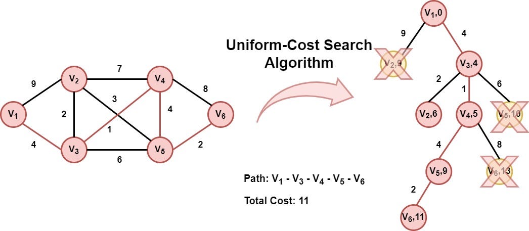
Uniform Cost Search

Uniform Cost Search (UCS) is a brute-force graph traversal algorithm used to find the path with the minimum cumulative cost from a source to a destination in a weighted graph. It is a type of uninformed search, meaning it doesn’t have any prior knowledge about the destination or heuristic guidance.

UCS functions similarly to Dijkstra’s algorithm. It expands the node with the lowest cost first using a priority queue where priority is determined by the cumulative cost to reach a node. It continues exploring the graph until it reaches the destination node with the least cost.

The algorithm uses a visited array to keep track of the explored nodes and ensures the shortest path is calculated without cycles. UCS is complete and optimal when all step costs are positive.

Time Complexity: Exponential in the worst case, especially when the minimum step cost ε is small relative to the optimal cost C. It is approximately O(b^C/ε) where b is the branching factor.

import java.util.PriorityQueue;
import java.util.*;

public class UniformCostSearch {

    private static final int INF = Integer.MAX_VALUE;

    public static int findShortestPath(int[][] edges, int n, int source, int destination) {
        PriorityQueue queue = new PriorityQueue<>((a, b) -> a.cost - b.cost);
        boolean[] visited = new boolean[n];
        HashMap> graph = new HashMap<>();

        for (int i = 0; i < n; i++) graph.put(i, new HashSet<>());
        for (int[] edge : edges) {
            graph.get(edge[0]).add(new Node(edge[1], edge[2]));
        }

        queue.add(new Node(source, 0));
        int minCost = INF;

        while (!queue.isEmpty()) {
            Node curNode = queue.poll();
            int cst = curNode.cost;

            if (curNode.vertex == destination) {
                minCost = Math.min(minCost, cst);
            } else {
                visited[curNode.vertex] = true;
                for (Node neighbor : graph.get(curNode.vertex)) {
                    if (!visited[neighbor.vertex]) {
                        queue.add(new Node(neighbor.vertex, neighbor.cost + cst));
                    }
                }
            }
        }

        return minCost;
    }

    private static class Node implements Comparable {
        int vertex, cost;
        public Node(int vertex, int cost) {
            this.vertex = vertex;
            this.cost = cost;
        }
        @Override
        public int compareTo(Node other) {
            return this.cost - other.cost;
        }
    }

    public static void main(String[] args) {
        int[][] graph = {
            {0, 3, 10}, {0, 1, 5}, {1, 5, 15},
            {1, 2, 4}, {2, 4, 8}, {3, 5, 11}, {5, 4, 4}
        };
        int source = 0;
        int destination = 4;
        int minCost = findShortestPath(graph, 6, source, destination);
        System.out.println("Minimum cost: " + minCost);
    }
}