System Design: Image Processing and Hemoglobin Prediction Pipeline

Step 1: White Balancing
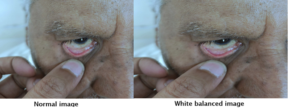
The first step corrects color distortions in the eye images by applying white balancing techniques to ensure consistent lighting and color representation.

// White Balancing Python Code
import cv2
import numpy as np
import os

METHOD = "gray_world"  # Options: "gray_world", "perfect_reflector", "histogram"

input_folder = r"C:\\Path\\To\\Input\\Images"
output_folder = r"C:\\Path\\To\\Output\\WhiteBalanced"

os.makedirs(output_folder, exist_ok=True)

def gray_world_white_balance(image):
    image = image.astype(np.float32)
    mean_r, mean_g, mean_b = np.mean(image[:,:,2]), np.mean(image[:,:,1]), np.mean(image[:,:,0])
    avg = (mean_r + mean_g + mean_b) / 3
    image[:,:,2] *= avg / mean_r
    image[:,:,1] *= avg / mean_g
    image[:,:,0] *= avg / mean_b
    return np.clip(image, 0, 255).astype(np.uint8)

for filename in os.listdir(input_folder):
    if filename.lower().endswith(('.png','.jpg','.jpeg')):
        image_path = os.path.join(input_folder, filename)
        image = cv2.imread(image_path)
        wb_image = gray_world_white_balance(image)
        cv2.imwrite(os.path.join(output_folder, filename), wb_image)

print("White balancing completed!")

Step 2: Image Annotation
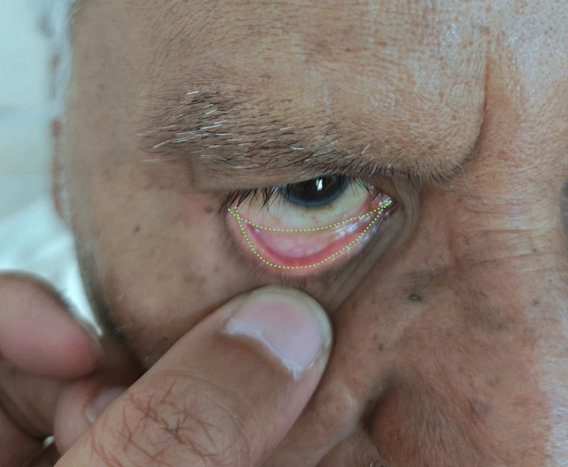
Next, each image is manually annotated by selecting points outlining the palpebral conjunctiva. This creates polygon masks used for training segmentation models.

# Image Annotation Code
import cv2
import os
import numpy as np

image_dir = "images"
output_dir = "output"
os.makedirs(output_dir, exist_ok=True)

points = []
original_image = None
image_display = None
image_name = ""
scale_factor = 0.5

def draw_polygon(event, x, y, flags, param):
    global points, image_display, original_image, scale_factor

    if event == cv2.EVENT_LBUTTONDOWN:
        x_orig, y_orig = int(x / scale_factor), int(y / scale_factor)
        points.append((x_orig, y_orig))
        cv2.circle(image_display, (x, y), 3, (0, 255, 0), -1)

    elif event == cv2.EVENT_RBUTTONDOWN:
        if len(points) > 2:
            cv2.polylines(image_display, [np.array(points) * scale_factor], isClosed=True, color=(0, 255, 0), thickness=2)
            save_annotation()
        points.clear()

# ... (rest of annotation code)

Step 3: Segmentation and Hemoglobin Prediction Model Training
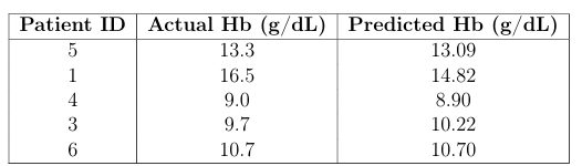
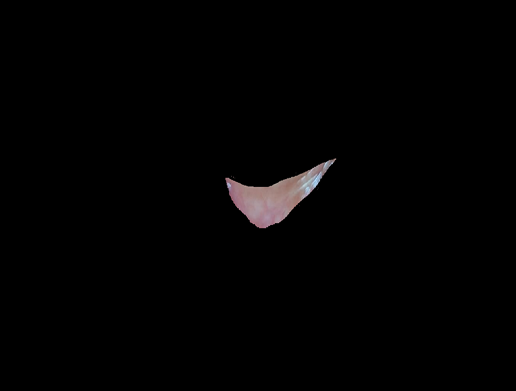
Using the annotated images, segmentation extracts the palpebral conjunctiva region. These segmented images, combined with patient metadata (age, sex, Hb levels), are used to train a hemoglobin level prediction model. We used a Random Forest Regressor to learn patterns from deep features extracted using MobileNetV2 along with patient metadata.

# Model Training Code
import pandas as pd
from sklearn.preprocessing import LabelEncoder
from sklearn.ensemble import RandomForestRegressor
from sklearn.model_selection import train_test_split
from sklearn.metrics import mean_squared_error, r2_score
import numpy as np
from tensorflow.keras.applications import MobileNetV2
from tensorflow.keras.preprocessing import image
from tensorflow.keras.applications.mobilenet_v2 import preprocess_input
import os

df = pd.read_excel("data.xlsx")
df.columns = df.columns.str.strip().str.lower().str.replace('.', '').str.replace(' ', '_')
df = df.dropna(subset=['hb'])
df['sex'] = LabelEncoder().fit_transform(df['sex'])

mobilenet = MobileNetV2(weights='imagenet', include_top=False, pooling='avg', input_shape=(224,224,3))

def extract_deep_features(img_path):
    # ... function body ...
    pass

# ... rest of model training ...

View Report