Introduction & Problem Statement
Last-mile delivery—getting packages from warehouses to customers—is one of the most challenging and costly parts of logistics. Issues like traffic, varied locations, and tight delivery windows make route planning tough. Traditional methods often cause delays, higher costs, and inefficient vehicle use.
Amazon uses systems like Condor to group orders and assign them efficiently to vehicles. For routing within these groups, algorithms like A* help find the best paths considering real-time traffic.
Combining order clustering, smart vehicle assignment, detailed routing, and machine learning for traffic and demand prediction creates a flexible, efficient delivery system. Real-time data lets routes adjust dynamically, reducing delivery time and costs while improving vehicle use and customer satisfaction..
Objectives
- To optimize last-mile delivery through efficient order clustering and vehicle assignment
- To plan optimal intra-cluster delivery routes using heuristic algorithms like A*
- To improve delivery planning with machine learning-based demand and traffic prediction
- To enable dynamic route adjustments using real-time traffic, weather, and vehicle data
System Flow Diagram
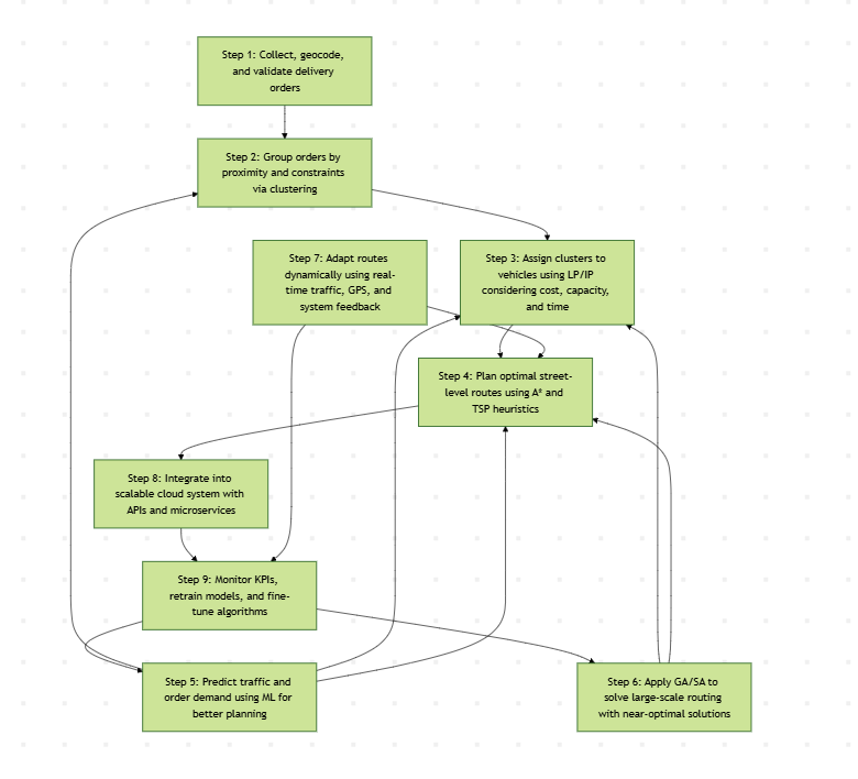
Proposed Solution
To build an efficient, scalable delivery system, we start by capturing real-time order data and organizing it through geographic clustering. We match these clusters to vehicles using optimization techniques that respect delivery windows and capacity limits. Routes within each cluster are planned using A* search, accounting for traffic and road constraints. Machine learning models help forecast demand and traffic to guide planning. For large-scale problems, metaheuristics like Genetic Algorithms are used to improve performance without sacrificing speed. The system integrates real-time data for dynamic re-routing and is deployed using a modular, cloud-based architecture. Continuous feedback and data-driven tuning help us improve efficiency, reduce delays, and scale with demand.
Step 1:
Real-Time Order Ingestion and Preprocessing
- Collect order details: Gather information like delivery addresses, delivery time windows, package size and weight, priority level, and delivery mode (bike, van, drone).
- Convert addresses to coordinates: Turn each delivery address into GPS coordinates (latitude and longitude) so locations can be mapped and processed.
- Validate orders: Check inventory to make sure items are available and remove any duplicate or incorrect orders.
Step 2: Geographic Clustering of Orders
- Group delivery orders into manageable clusters based on geographic proximity and delivery constraints.
- Use clustering algorithms such as k-means, DBSCAN, or hierarchical clustering:
- Input features for clustering include:
- Latitude and longitude of delivery addresses.
- Delivery time windows (converted to numerical values).
- Package size or weight, when vehicle capacity is a constraint.
- Clustering simplifies routing by dividing orders into smaller geographic zones.
- Ensures balanced workload and alignment with delivery time window constraints.
Step 3:
Vehicle Assignment Using Linear/Integer Programming (LP/IP)
- Assign each cluster of orders to the most suitable delivery vehicle.
- Define binary decision variables:
- x[v][c] = 1 if vehicle v is assigned to cluster c, otherwise 0.
- Minimize total cost → sum of (cost of assigning vehicle v to cluster c) × x[v][c].
- Cost can be distance, time, or fuel consumption.
- Minimize total cost → sum of (cost of assigning vehicle v to cluster c) × x[v][c].
- Cost can be distance, time, or fuel consumption.
- Each cluster is assigned to exactly one vehicle.
- Vehicle capacity limits (weight, volume) must not be exceeded.
- Deliveries must meet time windows.
- Route time or distance per vehicle must stay within limits.
- Use optimization tools like Gurobi, CPLEX, or open-source options like CBC or GLPK.
- For more flexibility, include soft constraints with penalties (e.g., slightly exceeding capacity at a cost).
Step 4:
Street-Level Route Planning Using A* Search
- For each assigned cluster, compute the detailed delivery route for the vehicle.
- Represent the road network as a weighted graph:
- Nodes represent intersections or delivery addresses.
- Edges represent roads with weights based on travel cost (like distance or time).
- Use the A* algorithm to find the optimal path between points:
- Apply heuristics like Euclidean or Manhattan distance to estimate the remaining cost.
- Use a cost function that adjusts travel time based on predicted traffic.
- For clusters with multiple stops, solve a variant of the Traveling Salesman Problem (TSP):
- Use heuristics like nearest neighbor or Christofides’ algorithm.
- Combine these with A* for computing path segments between stops.
- A* is effective for dynamic and accurate route planning, especially when traffic conditions vary in real-time.
Step 5: Demand and Traffic Prediction via Machine Learning
Predicting Demand and Traffic for Optimized Route Planning
- Use machine learning to forecast order demand and traffic conditions in advance.
- Demand Prediction:
- Apply time-series models like ARIMA or LSTM for forecasting.
- Use features such as historical order volumes, sales promotions, holidays, and seasonal trends.
- Traffic Prediction:
- Utilize real-time and historical traffic data with models like regression or neural networks.
- Incorporate features such as time of day, weather conditions, and road incidents.
- Apply Predictions to Optimize Planning:
- Adjust order clustering based on predicted high-demand areas.
- Optimize the number of vehicles and their capacities based on demand forecasts.
- Update travel times in the road network for the A* algorithm to route around predicted traffic congestion.
Step 6:
Metaheuristic Optimization for Large-Scale Scalability
- Large-scale delivery routing is a complex NP-hard problem that can’t always be solved exactly in a reasonable time.
- Use metaheuristic algorithms like Genetic Algorithms (GA) and Simulated Annealing (SA) to find good solutions fast.
- In Genetic Algorithms, create a set of possible routes, and improve them over time using operations like crossover and mutation.
- In Simulated Annealing, explore the solution space and sometimes accept less optimal solutions to avoid getting stuck in a bad spot.
- Start with a reasonable first solution using quick heuristics, like the Clarke-Wright savings method.
- Use results from earlier steps (like clustering and vehicle assignment) to limit the search space and guide the optimization.
- These methods help generate nearly optimal delivery routes even at Amazon’s massive scale, without needing enormous compute power.
Step 7:
Real-Time Data Integration & Dynamic Re-Routing
- Continuously gather real-time data from multiple sources like vehicle GPS, traffic services, weather updates, and warehouse inventory.
- Keep monitoring for any issues such as traffic jams, bad weather, or vehicle breakdowns.
- When something unexpected happens, quickly re-calculate new routes using A* for the affected deliveries.
- Send updated estimated arrival times (ETAs) to both drivers and customers.
- This real-time adjustment helps avoid delays, improves reliability, and keeps the delivery process smooth even when disruptions occur.
Step 8:
System Integration & Deployment
- Set up a data pipeline to stream incoming orders, vehicle location data, and external feeds like traffic and weather.
- Build an optimization engine that handles clustering, LP/IP assignment, demand forecasting, A* routing, and metaheuristic optimization.
- Create an API layer to send final route plans to delivery driver apps and internal dashboards.
- Add monitoring tools that track system performance and key delivery metrics for future improvements.
- Use a microservices architecture so each part (clustering, routing, etc.) can scale and update independently.
- Run the system on cloud infrastructure to easily handle changes in workload.
- Use caching and parallel processing to make the system fast and responsive.
Step 9:
Evaluation and Continuous Improvement
- Regularly measure key metrics like delivery cost per package, on-time rate, route length, planning time, and emissions.
- Collect and analyze performance data to identify areas that need improvement.
- Retrain machine learning models as more data comes in to keep predictions accurate.
- Fine-tune clustering methods and optimization heuristics based on results.
- Test out new strategies, algorithms, or hybrids to improve delivery efficiency over time.
Business Impact
- Real-time re-routing and traffic-aware planning improve delivery speed.
- Efficient clustering and routing reduce fuel usage and driver time.
- Continuous learning from real-time and historical data boosts performance.
Conclusion
The proposed system combines real-time data, machine learning, and intelligent optimization to streamline last-mile delivery. It reduces costs, improves delivery speed and accuracy, and scales efficiently—driving better customer experience and stronger business performance.
Download PDF